卷积自编码器
20 Apr 2018 | deep-learning |卷积自编码器
这一次我们使用基于卷积的自编码器,仍然使用MNIST数据集。
%matplotlib inline

import numpy as np
import tensorflow as tf
import matplotlib.pyplot as plt
from tensorflow.examples.tutorials.mnist import input_data
mnist = input_data.read_data_sets('MNIST_data', validation_size=0)
Extracting MNIST_data/train-images-idx3-ubyte.gz
Extracting MNIST_data/train-labels-idx1-ubyte.gz
Extracting MNIST_data/t10k-images-idx3-ubyte.gz
Extracting MNIST_data/t10k-labels-idx1-ubyte.gz
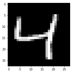
img = mnist.train.images[2]
plt.imshow(img.reshape((28, 28)), cmap='Greys_r')
<matplotlib.image.AxesImage at 0x7f4631f1a4e0>
网络架构
网络的编码器部分将是典型的卷积金字塔。每个卷积层之后将跟随有最大池化层以减小层的尺寸。解码器对你来说可能是陌生的。解码器需要从窄表示转换为宽表示,进而重构图像。例如,表示可以是4x4x8最大池化层。这是编码器的输出,同时作为解码器的输入。我们想从解码器得到一个28x28x1图像,所以我们需要从狭窄的解码器输入层返回。网络示意图如下所示。

这里,我们的最终编码器层的大小为4x4x8 = 128。原始图像具有尺寸28x28 = 784,因此编码向量大约是原始图像的尺寸的16%。这些只是每个层的建议尺寸。您可以随意更改深度和大小,但请记住,我们在这里的目标是找到小的输入数据表示。
解码器做了什么?
解码器有Upsample 层,可能你之前没有见过。通常,通过使用transposed convolution 来增加层的宽度和高度。这个与卷积操作很相似,只是反过来了。 例如,如果您有一个3x3内核,则输入层中的3x3将减少到卷积层中的一个单元。相比之下,输入层中的一个单元将扩展到转置卷积层中的3×3路径。TensorFlow 提供了这样的方法,我们可以直接使用, tf.nn.conv2d_transpose.
但是,转置卷积层会导致最终图像中的伪像,如棋盘图案。 这是由于内核的重叠,可以通过设置stride和kernel大小相等来避免。 在这篇文章中this Distill article ,作者展示了,如何避免该情况的发生. 在 TensorFlow, 很容易实现tf.image.resize_images。
inputs_ = tf.placeholder(tf.float32, (None, 28, 28, 1), name='inputs')
targets_ = tf.placeholder(tf.float32, (None, 28, 28, 1), name='targets')

### Encoder
conv1 = tf.layers.conv2d(inputs_, 16, (3,3), padding='same', activation=tf.nn.relu)
# Now 28x28x16
maxpool1 = tf.layers.max_pooling2d(conv1, (2,2), (2,2), padding='same')
# Now 14x14x16
conv2 = tf.layers.conv2d(maxpool1, 8, (3,3), padding='same', activation=tf.nn.relu)
# Now 14x14x8
maxpool2 = tf.layers.max_pooling2d(conv2, (2,2), (2,2), padding='same')
# Now 7x7x8
conv3 = tf.layers.conv2d(maxpool2, 8, (3,3), padding='same', activation=tf.nn.relu)
# Now 7x7x8
encoded = tf.layers.max_pooling2d(conv3, (2,2), (2,2), padding='same')
# Now 4x4x8

### Decoder
upsample1 = tf.image.resize_nearest_neighbor(encoded, (7,7))
# Now 7x7x8
conv4 = tf.layers.conv2d(upsample1, 8, (3,3), padding='same', activation=tf.nn.relu)
# Now 7x7x8
upsample2 = tf.image.resize_nearest_neighbor(conv4, (14,14))
# Now 14x14x8
conv5 = tf.layers.conv2d(upsample2, 8, (3,3), padding='same', activation=tf.nn.relu)
# Now 14x14x8
upsample3 = tf.image.resize_nearest_neighbor(conv5, (28,28))
# Now 28x28x8
conv6 = tf.layers.conv2d(upsample3, 16, (3,3), padding='same', activation=tf.nn.relu)
# Now 28x28x16

logits = tf.layers.conv2d(conv6, 1, (3,3), padding='same', activation=None)
#Now 28x28x1

decoded = tf.nn.sigmoid(logits, name='decoded')

loss = tf.nn.sigmoid_cross_entropy_with_logits(labels=targets_, logits=logits)
cost = tf.reduce_mean(loss)
opt = tf.train.AdamOptimizer(0.001).minimize(cost)
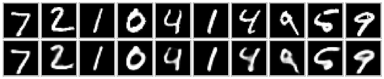
训练
和以前一样,这里我们将训练网络。我们可以将图像作为28x28x1传递输入,而不是平面化图像。
sess = tf.Session()
epochs = 20
batch_size = 200
sess.run(tf.global_variables_initializer())
for e in range(epochs):
    for ii in range(mnist.train.num_examples//batch_size):
        batch = mnist.train.next_batch(batch_size)
        imgs = batch[0].reshape((-1, 28, 28, 1))
        batch_cost, _ = sess.run([cost, opt], feed_dict={inputs_: imgs,
                                                         targets_: imgs})

        print("Epoch: {}/{}...".format(e+1, epochs),
              "Training loss: {:.4f}".format(batch_cost))
fig, axes = plt.subplots(nrows=2, ncols=10, sharex=True, sharey=True, figsize=(20,4))
in_imgs = mnist.test.images[:10]
reconstructed = sess.run(decoded, feed_dict={inputs_: in_imgs.reshape((10, 28, 28, 1))})

for images, row in zip([in_imgs, reconstructed], axes):
    for img, ax in zip(images, row):
        ax.imshow(img.reshape((28, 28)), cmap='Greys_r')
        ax.get_xaxis().set_visible(False)
        ax.get_yaxis().set_visible(False)


fig.tight_layout(pad=0.1)
sess.close()
降噪
正如之前所提到的,自动编码器在实践中并不太有用。然而,仅通过对噪声图像的网络训练,它们就可以成功地用于图像去噪。我们可以通过向训练图像添加高斯噪声,然后将这些值裁剪到0到1之间,来自己创建噪声图像。我们将使用噪声图像作为输入,而原始的干净图像作为目标。下面是噪声图像和去噪图像的示例。
 由于这对于网络来说是一个更困难的问题,我们希望在这里使用更深的卷积层,更多的特征映射。对于编码器中卷积层的深度,建议使用
32 - 32 - 16,同样的深度通过解码器。否则体系结构与以前相同。
inputs_ = tf.placeholder(tf.float32, (None, 28, 28, 1), name='inputs')
targets_ = tf.placeholder(tf.float32, (None, 28, 28, 1), name='targets')

### Encoder
conv1 = tf.layers.conv2d(inputs_, 32, (3,3), padding='same', activation=tf.nn.relu)
# Now 28x28x32
maxpool1 = tf.layers.max_pooling2d(conv1, (2,2), (2,2), padding='same')
# Now 14x14x32
conv2 = tf.layers.conv2d(maxpool1, 32, (3,3), padding='same', activation=tf.nn.relu)
# Now 14x14x32
maxpool2 = tf.layers.max_pooling2d(conv2, (2,2), (2,2), padding='same')
# Now 7x7x32
conv3 = tf.layers.conv2d(maxpool2, 16, (3,3), padding='same', activation=tf.nn.relu)
# Now 7x7x16
encoded = tf.layers.max_pooling2d(conv3, (2,2), (2,2), padding='same')
# Now 4x4x16

### Decoder
upsample1 = tf.image.resize_nearest_neighbor(encoded, (7,7))
# Now 7x7x16
conv4 = tf.layers.conv2d(upsample1, 16, (3,3), padding='same', activation=tf.nn.relu)
# Now 7x7x16
upsample2 = tf.image.resize_nearest_neighbor(conv4, (14,14))
# Now 14x14x16
conv5 = tf.layers.conv2d(upsample2, 32, (3,3), padding='same', activation=tf.nn.relu)
# Now 14x14x32
upsample3 = tf.image.resize_nearest_neighbor(conv5, (28,28))
# Now 28x28x32
conv6 = tf.layers.conv2d(upsample3, 32, (3,3), padding='same', activation=tf.nn.relu)
# Now 28x28x32

logits = tf.layers.conv2d(conv6, 1, (3,3), padding='same', activation=None)
#Now 28x28x1

decoded = tf.nn.sigmoid(logits, name='decoded')

loss = tf.nn.sigmoid_cross_entropy_with_logits(labels=targets_, logits=logits)
cost = tf.reduce_mean(loss)
opt = tf.train.AdamOptimizer(0.001).minimize(cost)
sess = tf.Session()
epochs = 100
batch_size = 200
# Set's how much noise we're adding to the MNIST images
noise_factor = 0.5
sess.run(tf.global_variables_initializer())
for e in range(epochs):
    for ii in range(mnist.train.num_examples//batch_size):
        batch = mnist.train.next_batch(batch_size)
        # Get images from the batch
        imgs = batch[0].reshape((-1, 28, 28, 1))

        # Add random noise to the input images
        noisy_imgs = imgs + noise_factor * np.random.randn(*imgs.shape)
        # Clip the images to be between 0 and 1
        noisy_imgs = np.clip(noisy_imgs, 0., 1.)

        # Noisy images as inputs, original images as targets
        batch_cost, _ = sess.run([cost, opt], feed_dict={inputs_: noisy_imgs,
                                                         targets_: imgs})

        print("Epoch: {}/{}...".format(e+1, epochs),
              "Training loss: {:.4f}".format(batch_cost))
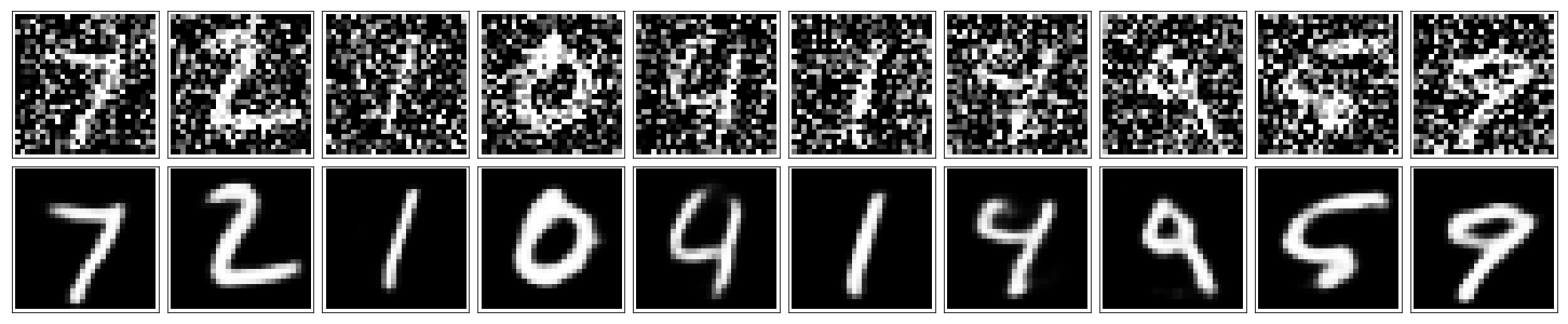
验证性能
Here I’m adding noise to the test images and passing them through the autoencoder. It does a suprising great job of removing the noise, even though it’s sometimes difficult to tell what the original number is.
fig, axes = plt.subplots(nrows=2, ncols=10, sharex=True, sharey=True, figsize=(20,4))
in_imgs = mnist.test.images[:10]
noisy_imgs = in_imgs + noise_factor * np.random.randn(*in_imgs.shape)
noisy_imgs = np.clip(noisy_imgs, 0., 1.)

reconstructed = sess.run(decoded, feed_dict={inputs_: noisy_imgs.reshape((10, 28, 28, 1))})

for images, row in zip([noisy_imgs, reconstructed], axes):
    for img, ax in zip(images, row):
        ax.imshow(img.reshape((28, 28)), cmap='Greys_r')
        ax.get_xaxis().set_visible(False)
        ax.get_yaxis().set_visible(False)

fig.tight_layout(pad=0.1)