批量归一化
01 Apr 2018 | deep-learning |批量归一化
什么是批量归一化?
批量归一化首次出现在 Sergey Ioffe’s 和 Christian Szegedy’s 2015年论文中 Batch Normalization: Accelerating Deep Network Training by Reducing Internal Covariate Shift. 其思想是不仅仅是对输入层进行归一化,而是对网络中的每一层输入都进行归一化操作。 叫做批量归一化的原因是:我们使用当前mini-batch的值的均值与偏差对每一层的输入都进行归一化。
为什么这样做会有效果呢?我们这知道对输入层做归一化有利于网络的学习。对网络中的每层而言,当前层的输出都会成为另一层的输入。那么我们可以这样来想:网络中的任何一层都可以作为接下来的网络的输入。例如,设想一个3层网络,不要把它看作是一个具有输入层、隐藏层和输出层的单个网络,而要把第1层的输出看作是接下来两层网络的输入,这个两层网络将由我们原始网络中的第2层和第3层组成。同样,第2层的输出可以被认为是对仅由第3层组成的单层网络的输入。
除了直观的原因之外,还有很好的数学原因可以帮助网络更好地学习。在这篇论文中有详细的解释,在深度学习 的第八章也有解释Chapter 8: Optimization for Training Deep Models.
批量归一化的好处
对网络进行批量归一化优化的好处是:
- 网络训练的更快 – 由于在训练期间的前向传播和方向传播需要处理更多的参数,实际上每次的迭代会慢一点;但是,它收敛会更加快速,所以总体上,网络的训练更快。
- 允许更高的学习率 – 梯度下降通常需要更小的学习率用于网络的训练。 随着网络的加深它需要更多的迭代次数。 使用批量归一化允许我们使用更高的学习速率,这进一步提高了网络训练的速度。
- 让权重更容易初始化 – 权重的初始化时困难的,特别是深层的网络。批量归一化让我在初始化权重时不需要那么小心。
- 让更多的激活函数具有可行性 – 有一些激活函数在某些情况下表现的不好。 Sigmoid函数会很快失去梯度,那么意味着它不能用在深层的网络。ReLUs函数经常在训练中死去(某些神经元变为了0),在那里他们完全停止学习,所以我们需要小心处理输入到节点值的范围.因为批量归一化调整了进入每个激活函数的值,所以在深层网络中那些似乎不能很好工作的非线性函数将再次变得可行。
- 简化深层网络的创建 – 因为批量归一化让更多的函数具有可行性,那么构建更加快速和深层的网络将会变得更加容易。
- 提供了一些正则化 – 批量归一化给网络增加了一些噪声,在某些情况下,它表现的和Dropout一样好。
- 总体或许会得到更好的结果 – 因为批量归一化可以让网络训练的更快,构建更深的网络,所以总体来说也会得到更好的结果。
在TensorFlow中实现批量归一化
首先我们需要导入MNIST数据集
# Import necessary packages
import tensorflow as tf
import tqdm
import numpy as np
import matplotlib.pyplot as plt
%matplotlib inline

# Import MNIST data so we have something for our experiments
from tensorflow.examples.tutorials.mnist import input_data
mnist = input_data.read_data_sets("MNIST_data/", one_hot=True)
Extracting MNIST_data/train-images-idx3-ubyte.gz
Extracting MNIST_data/train-labels-idx1-ubyte.gz
Extracting MNIST_data/t10k-images-idx3-ubyte.gz
Extracting MNIST_data/t10k-labels-idx1-ubyte.gz
创建用于测试的神经网络
NeuralNet类允许我们标记在网络中是否使用批量归一化。
注意:
该类的实现在TensorFlow中并不是最好的方式,这样做只是为了更好的讨论批量归一化。
在这个例子中我们使用了MNIST数据集,但是我们所创建的网络并不是一个好的识别手写数字体的方式,这样做同样只是为了更好的讨论批量归一化。
class NeuralNet:
    def __init__(self, initial_weights, activation_fn, use_batch_norm):
        """
        Initializes this object, creating a TensorFlow graph using the given parameters.

        :param initial_weights: list of NumPy arrays or Tensors
            Initial values for the weights for every layer in the network. We pass these in
            so we can create multiple networks with the same starting weights to eliminate
            training differences caused by random initialization differences.
            The number of items in the list defines the number of layers in the network,
            and the shapes of the items in the list define the number of nodes in each layer.
            e.g. Passing in 3 matrices of shape (784, 256), (256, 100), and (100, 10) would
            create a network with 784 inputs going into a hidden layer with 256 nodes,
            followed by a hidden layer with 100 nodes, followed by an output layer with 10 nodes.
        :param activation_fn: Callable
            The function used for the output of each hidden layer. The network will use the same
            activation function on every hidden layer and no activate function on the output layer.
            e.g. Pass tf.nn.relu to use ReLU activations on your hidden layers.
        :param use_batch_norm: bool
            Pass True to create a network that uses batch normalization; False otherwise
            Note: this network will not use batch normalization on layers that do not have an
            activation function.
        """
        # Keep track of whether or not this network uses batch normalization.
        self.use_batch_norm = use_batch_norm
        self.name = "With Batch Norm" if use_batch_norm else "Without Batch Norm"

        # Batch normalization needs to do different calculations during training and inference,
        # so we use this placeholder to tell the graph which behavior to use.
        self.is_training = tf.placeholder(tf.bool, name="is_training")

        # This list is just for keeping track of data we want to plot later.
        # It doesn't actually have anything to do with neural nets or batch normalization.
        self.training_accuracies = []

        # Create the network graph, but it will not actually have any real values until after you
        # call train or test
        self.build_network(initial_weights, activation_fn)

    def build_network(self, initial_weights, activation_fn):
        """
        Build the graph. The graph still needs to be trained via the `train` method.

        :param initial_weights: list of NumPy arrays or Tensors
            See __init__ for description.
        :param activation_fn: Callable
            See __init__ for description.
        """
        self.input_layer = tf.placeholder(tf.float32, [None, initial_weights[0].shape[0]])
        layer_in = self.input_layer
        for weights in initial_weights[:-1]:
            layer_in = self.fully_connected(layer_in, weights, activation_fn)
        self.output_layer = self.fully_connected(layer_in, initial_weights[-1])

    def fully_connected(self, layer_in, initial_weights, activation_fn=None):
        """
        Creates a standard, fully connected layer. Its number of inputs and outputs will be
        defined by the shape of `initial_weights`, and its starting weight values will be
        taken directly from that same parameter. If `self.use_batch_norm` is True, this
        layer will include batch normalization, otherwise it will not.

        :param layer_in: Tensor
            The Tensor that feeds into this layer. It's either the input to the network or the output
            of a previous layer.
        :param initial_weights: NumPy array or Tensor
            Initial values for this layer's weights. The shape defines the number of nodes in the layer.
            e.g. Passing in 3 matrix of shape (784, 256) would create a layer with 784 inputs and 256
            outputs.
        :param activation_fn: Callable or None (default None)
            The non-linearity used for the output of the layer. If None, this layer will not include
            batch normalization, regardless of the value of `self.use_batch_norm`.
            e.g. Pass tf.nn.relu to use ReLU activations on your hidden layers.
        """
        # Since this class supports both options, only use batch normalization when
        # requested. However, do not use it on the final layer, which we identify
        # by its lack of an activation function.
        if self.use_batch_norm and activation_fn:
            # Batch normalization uses weights as usual, but does NOT add a bias term. This is because
            # its calculations include gamma and beta variables that make the bias term unnecessary.
            # (See later in the notebook for more details.)
            weights = tf.Variable(initial_weights)
            linear_output = tf.matmul(layer_in, weights)

            # Apply batch normalization to the linear combination of the inputs and weights
            batch_normalized_output = tf.layers.batch_normalization(linear_output, training=self.is_training)

            # Now apply the activation function, *after* the normalization.
            return activation_fn(batch_normalized_output)
        else:
            # When not using batch normalization, create a standard layer that multiplies
            # the inputs and weights, adds a bias, and optionally passes the result
            # through an activation function.
            weights = tf.Variable(initial_weights)
            biases = tf.Variable(tf.zeros([initial_weights.shape[-1]]))
            linear_output = tf.add(tf.matmul(layer_in, weights), biases)
            return linear_output if not activation_fn else activation_fn(linear_output)

    def train(self, session, learning_rate, training_batches, batches_per_sample, save_model_as=None):
        """
        Trains the model on the MNIST training dataset.

        :param session: Session
            Used to run training graph operations.
        :param learning_rate: float
            Learning rate used during gradient descent.
        :param training_batches: int
            Number of batches to train.
        :param batches_per_sample: int
            How many batches to train before sampling the validation accuracy.
        :param save_model_as: string or None (default None)
            Name to use if you want to save the trained model.
        """
        # This placeholder will store the target labels for each mini batch
        labels = tf.placeholder(tf.float32, [None, 10])

        # Define loss and optimizer
        cross_entropy = tf.reduce_mean(
            tf.nn.softmax_cross_entropy_with_logits(labels=labels, logits=self.output_layer))

        # Define operations for testing
        correct_prediction = tf.equal(tf.argmax(self.output_layer, 1), tf.argmax(labels, 1))
        accuracy = tf.reduce_mean(tf.cast(correct_prediction, tf.float32))

        if self.use_batch_norm:
            # If we don't include the update ops as dependencies on the train step, the
            # tf.layers.batch_normalization layers won't update their population statistics,
            # which will cause the model to fail at inference time
            with tf.control_dependencies(tf.get_collection(tf.GraphKeys.UPDATE_OPS)):
                train_step = tf.train.GradientDescentOptimizer(learning_rate).minimize(cross_entropy)
        else:
            train_step = tf.train.GradientDescentOptimizer(learning_rate).minimize(cross_entropy)

        # Train for the appropriate number of batches. (tqdm is only for a nice timing display)
        for i in tqdm.tqdm(range(training_batches)):
            # We use batches of 60 just because the original paper did. You can use any size batch you like.
            batch_xs, batch_ys = mnist.train.next_batch(60)
            session.run(train_step, feed_dict={self.input_layer: batch_xs,
                                               labels: batch_ys,
                                               self.is_training: True})

            # Periodically test accuracy against the 5k validation images and store it for plotting later.
            if i % batches_per_sample == 0:
                test_accuracy = session.run(accuracy, feed_dict={self.input_layer: mnist.validation.images,
                                                                 labels: mnist.validation.labels,
                                                                 self.is_training: False})
                self.training_accuracies.append(test_accuracy)

        # After training, report accuracy against test data
        test_accuracy = session.run(accuracy, feed_dict={self.input_layer: mnist.validation.images,
                                                         labels: mnist.validation.labels,
                                                         self.is_training: False})
        print('{}: After training, final accuracy on validation set = {}'.format(self.name, test_accuracy))

        # If you want to use this model later for inference instead of having to retrain it,
        # just construct it with the same parameters and then pass this file to the 'test' function
        if save_model_as:
            tf.train.Saver().save(session, save_model_as)

    def test(self, session, test_training_accuracy=False, include_individual_predictions=False, restore_from=None):
        """
        Trains a trained model on the MNIST testing dataset.

        :param session: Session
            Used to run the testing graph operations.
        :param test_training_accuracy: bool (default False)
            If True, perform inference with batch normalization using batch mean and variance;
            if False, perform inference with batch normalization using estimated population mean and variance.
            Note: in real life, *always* perform inference using the population mean and variance.
                  This parameter exists just to support demonstrating what happens if you don't.
        :param include_individual_predictions: bool (default True)
            This function always performs an accuracy test against the entire test set. But if this parameter
            is True, it performs an extra test, doing 200 predictions one at a time, and displays the results
            and accuracy.
        :param restore_from: string or None (default None)
            Name of a saved model if you want to test with previously saved weights.
        """
        # This placeholder will store the true labels for each mini batch
        labels = tf.placeholder(tf.float32, [None, 10])

        # Define operations for testing
        correct_prediction = tf.equal(tf.argmax(self.output_layer, 1), tf.argmax(labels, 1))
        accuracy = tf.reduce_mean(tf.cast(correct_prediction, tf.float32))

        # If provided, restore from a previously saved model
        if restore_from:
            tf.train.Saver().restore(session, restore_from)

        # Test against all of the MNIST test data
        test_accuracy = session.run(accuracy, feed_dict={self.input_layer: mnist.test.images,
                                                         labels: mnist.test.labels,
                                                         self.is_training: test_training_accuracy})
        print('-'*75)
        print('{}: Accuracy on full test set = {}'.format(self.name, test_accuracy))

        # If requested, perform tests predicting individual values rather than batches
        if include_individual_predictions:
            predictions = []
            correct = 0

            # Do 200 predictions, 1 at a time
            for i in range(200):
                # This is a normal prediction using an individual test case. However, notice
                # we pass `test_training_accuracy` to `feed_dict` as the value for `self.is_training`.
                # Remember that will tell it whether it should use the batch mean & variance or
                # the population estimates that were calucated while training the model.
                pred, corr = session.run([tf.arg_max(self.output_layer,1), accuracy],
                                         feed_dict={self.input_layer: [mnist.test.images[i]],
                                                    labels: [mnist.test.labels[i]],
                                                    self.is_training: test_training_accuracy})
                correct += corr

                predictions.append(pred[0])

            print("200 Predictions:", predictions)
            print("Accuracy on 200 samples:", correct/200)
在代码中添加了许多的注释,应该能够解答你许多疑惑,接下来我们看看其中重要的代码。
在 fully_connected 函数中我们添加了批量归一化函数。有几点我们需要注意:
- 批量归一化层并不包括偏差项
- 我们使用TensorFlow’s
tf.layers.batch_normalization函数来处理其中的数学计算。 (稍后我们也会实现低版本的批量归一化 later in the notebook.) - 我们需要让
tf.layers.batch_normalization函数知道我们是否处于训练阶段。 - 在激活函数之前我们进行的批量归一化操作
还有一个函数我们需要注意:
with tf.control_dependencies(tf.get_collection(tf.GraphKeys.UPDATE_OPS)):
如果没有这一行,TensorFlow的批量归一化层在推理期间将不会正常工作。
我们需要在训练或者推理阶段分别传入True和False。
session.run(train_step, feed_dict={self.input_layer: batch_xs,
                                               labels: batch_ys,
                                               self.is_training: True})
批量归一化例子
这一节我们将会以实验来说明批量归一化的好处。
参考博文: Implementing Batch Normalization in TensorFlow.
辅助代码
第一个函数 plot_training_accuracies, 用于绘制传入到NeuralNet类中的training_accuracies的值。
第二个函数 train_and_test,创建了两个神经网络,一个使用批量归一化,一个不使用。 一个用于训练,一个用于测试,它会调用plot_training_accuracies函数绘制在训练过程中准确度的变化。更重要的是,使用的是相同的初始化权重,消除了不同权重所造成的性能影响。
def plot_training_accuracies(*args, **kwargs):
    """
    Displays a plot of the accuracies calculated during training to demonstrate
    how many iterations it took for the model(s) to converge.

    :param args: One or more NeuralNet objects
        You can supply any number of NeuralNet objects as unnamed arguments
        and this will display their training accuracies. Be sure to call `train`
        the NeuralNets before calling this function.
    :param kwargs:
        You can supply any named parameters here, but `batches_per_sample` is the only
        one we look for. It should match the `batches_per_sample` value you passed
        to the `train` function.
    """
    fig, ax = plt.subplots()

    batches_per_sample = kwargs['batches_per_sample']

    for nn in args:
        ax.plot(range(0,len(nn.training_accuracies)*batches_per_sample,batches_per_sample),
                nn.training_accuracies, label=nn.name)
    ax.set_xlabel('Training steps')
    ax.set_ylabel('Accuracy')
    ax.set_title('Validation Accuracy During Training')
    ax.legend(loc=4)
    ax.set_ylim([0,1])
    plt.yticks(np.arange(0, 1.1, 0.1))
    plt.grid(True)
    plt.show()

def train_and_test(use_bad_weights, learning_rate, activation_fn, training_batches=50000, batches_per_sample=500):
    """
    Creates two networks, one with and one without batch normalization, then trains them
    with identical starting weights, layers, batches, etc. Finally tests and plots their accuracies.

    :param use_bad_weights: bool
        If True, initialize the weights of both networks to wildly inappropriate weights;
        if False, use reasonable starting weights.
    :param learning_rate: float
        Learning rate used during gradient descent.
    :param activation_fn: Callable
        The function used for the output of each hidden layer. The network will use the same
        activation function on every hidden layer and no activate function on the output layer.
        e.g. Pass tf.nn.relu to use ReLU activations on your hidden layers.
    :param training_batches: (default 50000)
        Number of batches to train.
    :param batches_per_sample: (default 500)
        How many batches to train before sampling the validation accuracy.
    """
    # Use identical starting weights for each network to eliminate differences in
    # weight initialization as a cause for differences seen in training performance
    #
    # Note: The networks will use these weights to define the number of and shapes of
    #       its layers. The original batch normalization paper used 3 hidden layers
    #       with 100 nodes in each, followed by a 10 node output layer. These values
    #       build such a network, but feel free to experiment with different choices.
    #       However, the input size should always be 784 and the final output should be 10.
    if use_bad_weights:
        # These weights should be horrible because they have such a large standard deviation
        weights = [np.random.normal(size=(784,100), scale=5.0).astype(np.float32),
                   np.random.normal(size=(100,100), scale=5.0).astype(np.float32),
                   np.random.normal(size=(100,100), scale=5.0).astype(np.float32),
                   np.random.normal(size=(100,10), scale=5.0).astype(np.float32)
                  ]
    else:
        # These weights should be good because they have such a small standard deviation
        weights = [np.random.normal(size=(784,100), scale=0.05).astype(np.float32),
                   np.random.normal(size=(100,100), scale=0.05).astype(np.float32),
                   np.random.normal(size=(100,100), scale=0.05).astype(np.float32),
                   np.random.normal(size=(100,10), scale=0.05).astype(np.float32)
                  ]

    # Just to make sure the TensorFlow's default graph is empty before we start another
    # test, because we don't bother using different graphs or scoping and naming
    # elements carefully in this sample code.
    tf.reset_default_graph()

    # build two versions of same network, 1 without and 1 with batch normalization
    nn = NeuralNet(weights, activation_fn, False)
    bn = NeuralNet(weights, activation_fn, True)

    # train and test the two models
    with tf.Session() as sess:
        tf.global_variables_initializer().run()

        nn.train(sess, learning_rate, training_batches, batches_per_sample)
        bn.train(sess, learning_rate, training_batches, batches_per_sample)

        nn.test(sess)
        bn.test(sess)

    # Display a graph of how validation accuracies changed during training
    # so we can compare how the models trained and when they converged
    plot_training_accuracies(nn, bn, batches_per_sample=batches_per_sample)
比较两个网络
接下来会创建两个神经网络,他们使用ReLU作激活函数,0.01的学习率和合理的初始化权重值
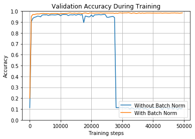
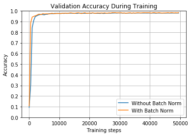
train_and_test(False, 0.01, tf.nn.relu)
100%|███████████████████████████████████| 50000/50000 [02:49<00:00, 295.09it/s]


Without Batch Norm: After training, final accuracy on validation set = 0.9728000164031982


100%|███████████████████████████████████| 50000/50000 [05:10<00:00, 160.97it/s]


With Batch Norm: After training, final accuracy on validation set = 0.9818000197410583
---------------------------------------------------------------------------
Without Batch Norm: Accuracy on full test set = 0.9704999923706055
---------------------------------------------------------------------------
With Batch Norm: Accuracy on full test set = 0.9775999784469604
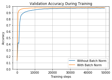
正如你所见,两个网络最终的准确度都差不多,但是,进行批量归一化操作的网络收敛的更快,大约在10000次的迭代中,而另一个大约在30000次迭代中才收敛。
如果你看了原始的训练速度,会注意到,没有进行批量归一化的网络每秒可以处理1100个batch,而进行批量归一化处理的网络每秒只能处理500个batch,但是它收敛的更快。
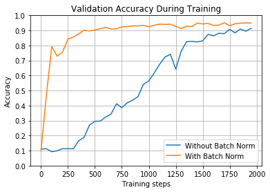
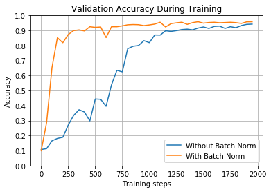
接下来的网络使用的参数与之前相同,但是只是迭代了2000次
train_and_test(False, 0.01, tf.nn.relu, 2000, 50)
100%|█████████████████████████████████████| 2000/2000 [00:08<00:00, 230.00it/s]


Without Batch Norm: After training, final accuracy on validation set = 0.8352000117301941


100%|█████████████████████████████████████| 2000/2000 [00:16<00:00, 123.99it/s]


With Batch Norm: After training, final accuracy on validation set = 0.953000009059906
---------------------------------------------------------------------------
Without Batch Norm: Accuracy on full test set = 0.8278999924659729
---------------------------------------------------------------------------
With Batch Norm: Accuracy on full test set = 0.9516000151634216
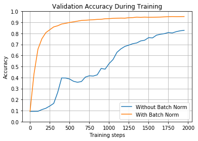
如图所示,使用批量归一化的网络仅仅用了2000个batch就达到了95%的准确度,500个batch就达到了90%的准确度;而没有使用批量归一化的网络用了1750个batch才达到了85%.(注意,你自己训练时,由于权重的随机性,数值可能有一些差异)
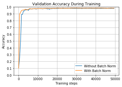
接下来创建的两个神经网络,他们使用sigmoid作激活函数,0.01的学习率和合理的初始化权重值.
train_and_test(False, 0.01, tf.nn.sigmoid)
100%|██████████| 50000/50000 [00:43<00:00, 1153.97it/s]


Without Batch Norm: After training, final accuracy on validation set = 0.8343997597694397


100%|██████████| 50000/50000 [01:35<00:00, 526.30it/s]


With Batch Norm: After training, final accuracy on validation set = 0.9755997061729431
---------------------------------------------------------------------------
Without Batch Norm: Accuracy on full test set = 0.8271000385284424
---------------------------------------------------------------------------
With Batch Norm: Accuracy on full test set = 0.9732001423835754
从上图中,我们也可以明显看出批量归一化的网络的性能很不错。
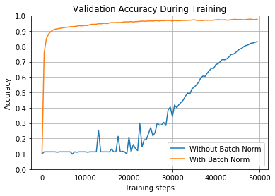
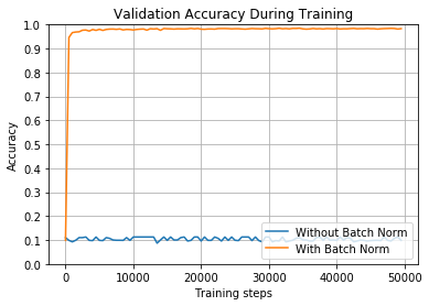
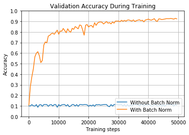
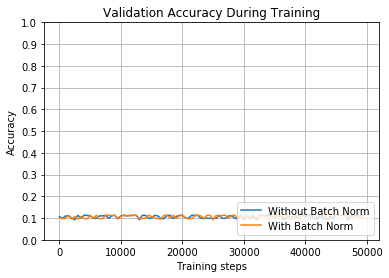
接下来创建的两个神经网络,他们使用ReLU作激活函数,1的学习率和合理的初始化权重值
train_and_test(False, 1, tf.nn.relu)
100%|██████████| 50000/50000 [00:35<00:00, 1397.55it/s]


Without Batch Norm: After training, final accuracy on validation set = 0.0957999974489212


100%|██████████| 50000/50000 [01:39<00:00, 501.48it/s]


With Batch Norm: After training, final accuracy on validation set = 0.984399676322937
---------------------------------------------------------------------------
Without Batch Norm: Accuracy on full test set = 0.09799998998641968
---------------------------------------------------------------------------
With Batch Norm: Accuracy on full test set = 0.9834001660346985
现在我们再次使用ReLU,但学习率更高一些。该图显示了开始训练是正常,批量归一化的网络比其他网络开始得更快。但是,较高的学习率会使准确度反弹得更厉害,在某个时候,没有批量归一化的网络中的准确度会完全崩溃。很可能是因为高学习率,太多的ReLU在这个时候死了。
train_and_test(False, 1, tf.nn.relu)
100%|██████████| 50000/50000 [00:36<00:00, 1379.92it/s]


Without Batch Norm: After training, final accuracy on validation set = 0.09859999269247055


100%|██████████| 50000/50000 [01:42<00:00, 488.08it/s]


With Batch Norm: After training, final accuracy on validation set = 0.9839996695518494
---------------------------------------------------------------------------
Without Batch Norm: Accuracy on full test set = 0.10099999606609344
---------------------------------------------------------------------------
With Batch Norm: Accuracy on full test set = 0.9822001457214355
在前面的两个示例中,具有批量归一化的网络能够获得98%以上的准确度,并且几乎立即接近该结果。较高的学习率使网络训练速度极快。
接下来创建的两个神经网络,他们使用sigmoid作激活函数,1的学习率和合理的初始化权重值
train_and_test(False, 1, tf.nn.sigmoid)
100%|██████████| 50000/50000 [00:36<00:00, 1382.38it/s]


Without Batch Norm: After training, final accuracy on validation set = 0.9783996343612671


100%|██████████| 50000/50000 [01:35<00:00, 526.13it/s]


With Batch Norm: After training, final accuracy on validation set = 0.9837996959686279
---------------------------------------------------------------------------
Without Batch Norm: Accuracy on full test set = 0.9752001166343689
---------------------------------------------------------------------------
With Batch Norm: Accuracy on full test set = 0.981200098991394
在本例中,我们切换到sigmoid激活函数。它似乎很好地处理了较高的学习率,两个网络都达到了高精度。
train_and_test(False, 1, tf.nn.sigmoid, 2000, 50)
100%|██████████| 2000/2000 [00:01<00:00, 1167.28it/s]


Without Batch Norm: After training, final accuracy on validation set = 0.920799732208252


100%|██████████| 2000/2000 [00:04<00:00, 490.92it/s]


With Batch Norm: After training, final accuracy on validation set = 0.951799750328064
---------------------------------------------------------------------------
Without Batch Norm: Accuracy on full test set = 0.9227001070976257
---------------------------------------------------------------------------
With Batch Norm: Accuracy on full test set = 0.9463001489639282
正如您所看到的,尽管这些参数对两个网络都很有效,但批量归一化的参数在400个左右的批处理中达到90%以上,而另一个参数则超过1700个。当训练更大的网络时,这种差异变得更加明显。
接下来创建的两个神经网络,他们使用ReLu作激活函数,学习率为2和合理的初始化权重值
train_and_test(False, 2, tf.nn.relu)
100%|██████████| 50000/50000 [00:35<00:00, 1412.09it/s]


Without Batch Norm: After training, final accuracy on validation set = 0.09859999269247055


100%|██████████| 50000/50000 [01:36<00:00, 518.06it/s]


With Batch Norm: After training, final accuracy on validation set = 0.9827996492385864
---------------------------------------------------------------------------
Without Batch Norm: Accuracy on full test set = 0.10099999606609344
---------------------------------------------------------------------------
With Batch Norm: Accuracy on full test set = 0.9827001094818115
利用这种非常大的学习率,具有批量归一化的网络训练更加精准,并且几乎立即达到98%的准确度。但是,没有归一化的网络根本无法学习。
接下来创建的两个神经网络,他们使用sigmoid作激活函数,学习率为2和合理的初始化权重值
train_and_test(False, 2, tf.nn.sigmoid)
100%|██████████| 50000/50000 [00:35<00:00, 1395.37it/s]


Without Batch Norm: After training, final accuracy on validation set = 0.9795997142791748


100%|██████████| 50000/50000 [01:38<00:00, 506.05it/s]


With Batch Norm: After training, final accuracy on validation set = 0.9803997278213501
---------------------------------------------------------------------------
Without Batch Norm: Accuracy on full test set = 0.9782001376152039
---------------------------------------------------------------------------
With Batch Norm: Accuracy on full test set = 0.9782000780105591
再一次,使用具有较大学习速率的sigmoid激活函数在批量归一化和不批量归一化的情况下都能很好地工作。
但是,看下面的图,其中我们训练的模型具有相同的参数,但只有2000次迭代。与往常一样,批量归一化使其训练更快。
train_and_test(False, 2, tf.nn.sigmoid, 2000, 50)
100%|██████████| 2000/2000 [00:01<00:00, 1170.27it/s]


Without Batch Norm: After training, final accuracy on validation set = 0.9383997917175293


100%|██████████| 2000/2000 [00:04<00:00, 495.04it/s]


With Batch Norm: After training, final accuracy on validation set = 0.9573997259140015
---------------------------------------------------------------------------
Without Batch Norm: Accuracy on full test set = 0.9360001087188721
---------------------------------------------------------------------------
With Batch Norm: Accuracy on full test set = 0.9524001479148865
在接下来的例子中,我们使用的起始权重非常差。也就是说,通常我们使用非常小的接近于零的值。但是,在这些示例中,我们选择标准偏差为5的随机值。如果你真的在训练一个神经网络,你并不会选择这样做。但是这些示例演示了批量归一化如何使您的网络更具弹性。
接下来创建的两个神经网络,他们使用ReLU作激活函数,学习率为0.01和糟糕的初始化权重值.
train_and_test(True, 0.01, tf.nn.relu)
100%|██████████| 50000/50000 [00:43<00:00, 1147.21it/s]


Without Batch Norm: After training, final accuracy on validation set = 0.0957999974489212


100%|██████████| 50000/50000 [01:37<00:00, 515.05it/s]


With Batch Norm: After training, final accuracy on validation set = 0.7945998311042786
---------------------------------------------------------------------------
Without Batch Norm: Accuracy on full test set = 0.09799998998641968
---------------------------------------------------------------------------
With Batch Norm: Accuracy on full test set = 0.7990000247955322
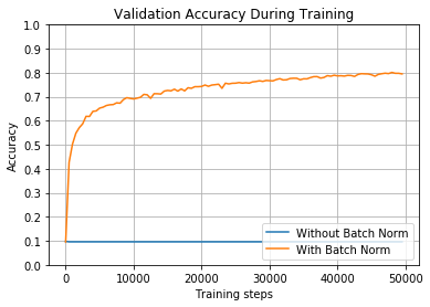
如图所示,如果不进行批量归一化化,网络将永远无法了解任何内容。但是,通过批量归一化,它实际上学习得相当好,准确率达到了近80%。起始权重显然会损害网络,但您可以看到批量归一化在克服它们方面所取得的效果。
接下来创建的两个神经网络,他们使用sigmoid作激活函数,学习率为0.01和糟糕的初始化权重值.
train_and_test(True, 0.01, tf.nn.sigmoid)
100%|██████████| 50000/50000 [00:45<00:00, 1108.50it/s]


Without Batch Norm: After training, final accuracy on validation set = 0.22019998729228973


100%|██████████| 50000/50000 [01:34<00:00, 531.21it/s]


With Batch Norm: After training, final accuracy on validation set = 0.8591998219490051
---------------------------------------------------------------------------
Without Batch Norm: Accuracy on full test set = 0.22699999809265137
---------------------------------------------------------------------------
With Batch Norm: Accuracy on full test set = 0.8527000546455383
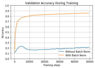
在前面的示例中,使用sigmoid激活函数比ReLU工作得更好,但是如果不进行批量归一化,则训练网络将需要非常长的时间。
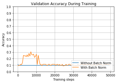
接下来创建的两个神经网络,他们使用ReLud作激活函数,学习率为1和糟糕的初始化权重值.
train_and_test(True, 1, tf.nn.relu)
100%|██████████| 50000/50000 [00:38<00:00, 1313.14it/s]


Without Batch Norm: After training, final accuracy on validation set = 0.11259999126195908


100%|██████████| 50000/50000 [01:36<00:00, 520.39it/s]


With Batch Norm: After training, final accuracy on validation set = 0.9243997931480408
---------------------------------------------------------------------------
Without Batch Norm: Accuracy on full test set = 0.11349999904632568
---------------------------------------------------------------------------
With Batch Norm: Accuracy on full test set = 0.9208000302314758
此处使用的较高学习速率允许批量归一化的网络在大约3万个batch中超过90%。而没有使用归一化的网络永远无法到达任何地方。
接下来创建的两个神经网络,他们使用sigmoid作激活函数,学习率为1和糟糕的初始化权重值.
train_and_test(True, 1, tf.nn.sigmoid)
100%|██████████| 50000/50000 [00:35<00:00, 1409.45it/s]


Without Batch Norm: After training, final accuracy on validation set = 0.896999716758728


100%|██████████| 50000/50000 [01:33<00:00, 534.39it/s]


With Batch Norm: After training, final accuracy on validation set = 0.9569997787475586
---------------------------------------------------------------------------
Without Batch Norm: Accuracy on full test set = 0.8957001566886902
---------------------------------------------------------------------------
With Batch Norm: Accuracy on full test set = 0.9505001306533813
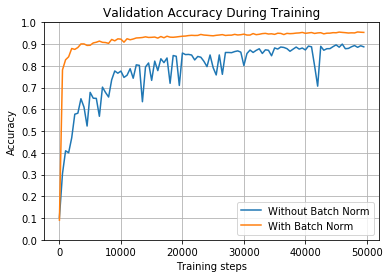
使用sigmoid比ReLU更有利于提高学习率。但是,您可以看到,如果不进行批量归一化,网络将需要很长时间的训练、来回颠簸,并且会在90%的时间内停滞不前。采用批量归一化的网络训练速度更快,稳定性更好,精度更高。
接下来创建的两个神经网络,他们使用ReLU作激活函数,学习率为2和糟糕的初始化权重值.
train_and_test(True, 2, tf.nn.relu)
100%|██████████| 50000/50000 [00:35<00:00, 1392.83it/s]


Without Batch Norm: After training, final accuracy on validation set = 0.0957999974489212


100%|██████████| 50000/50000 [01:33<00:00, 536.51it/s]


With Batch Norm: After training, final accuracy on validation set = 0.9127997159957886
---------------------------------------------------------------------------
Without Batch Norm: Accuracy on full test set = 0.09800000488758087
---------------------------------------------------------------------------
With Batch Norm: Accuracy on full test set = 0.9054000973701477
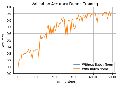
我们已经看到,ReLU在学习率上不如sigmoid,我们现在使用的是极高的学习率。正如预期的那样,如果没有批量归一化,网络根本无法学习。但通过批量归一化,最终达到90%的准确率。不过,请注意,它的准确性在训练中如何剧烈波动——这是因为学习率实在太高了,所以这一点起作用的是有点运气。
接下来创建的两个神经网络,他们使用sigmoid作激活函数,学习率为2和糟糕的初始化权重值.
train_and_test(True, 2, tf.nn.sigmoid)
100%|██████████| 50000/50000 [00:35<00:00, 1401.19it/s]


Without Batch Norm: After training, final accuracy on validation set = 0.9093997478485107


100%|██████████| 50000/50000 [01:33<00:00, 532.22it/s]


With Batch Norm: After training, final accuracy on validation set = 0.9613996744155884
---------------------------------------------------------------------------
Without Batch Norm: Accuracy on full test set = 0.9066000580787659
---------------------------------------------------------------------------
With Batch Norm: Accuracy on full test set = 0.9583001136779785
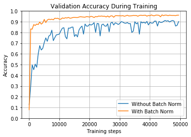
在这种情况下,具有批量归一化的网络训练速度更快,精度更高。同时,高的学习率使得没有归一化的网络在不规则的情况下反弹,并且难以达到90%以上。
批处理归一化化并不能解决所有问题
批量归一化并不是魔术,也不是每次都能奏效。权重仍然是随机初始化的,并且在训练期间随机选择批次,因此您永远不知道训练将如何进行。即使在这些测试中,我们对两个网络使用相同的初始权重,每次运行时我们仍然得到不同的权重。 本节包括两个示例,显示批量归一化完全没有起作用。
接下来创建的两个神经网络,他们使用ReLU作激活函数,学习率为1和糟糕的初始化权重值..
train_and_test(True, 1, tf.nn.relu)
100%|██████████| 50000/50000 [00:36<00:00, 1386.17it/s]


Without Batch Norm: After training, final accuracy on validation set = 0.11259999126195908


100%|██████████| 50000/50000 [01:35<00:00, 523.58it/s]


With Batch Norm: After training, final accuracy on validation set = 0.09879998862743378
---------------------------------------------------------------------------
Without Batch Norm: Accuracy on full test set = 0.11350000649690628
---------------------------------------------------------------------------
With Batch Norm: Accuracy on full test set = 0.10099999606609344
当我们早先使用这些相同的参数earlier时,我们看到批量归一化的网络达到92%的验证精度。这一次我们使用了不同的起始权重,使用与以前相同的标准偏差进行初始化,而网络根本无法学习。(请记住,如果网络总是猜测相同的值,那么其准确度大约为10%。)
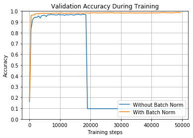
接下来创建的两个神经网络,他们使用ReLU作激活函数,学习率为2和糟糕的初始化权重值..
train_and_test(True, 2, tf.nn.relu)
100%|██████████| 50000/50000 [00:35<00:00, 1398.39it/s]


Without Batch Norm: After training, final accuracy on validation set = 0.0957999974489212


100%|██████████| 50000/50000 [01:34<00:00, 529.50it/s]


With Batch Norm: After training, final accuracy on validation set = 0.09859999269247055
---------------------------------------------------------------------------
Without Batch Norm: Accuracy on full test set = 0.09799998998641968
---------------------------------------------------------------------------
With Batch Norm: Accuracy on full test set = 0.10100000351667404
当我们用这些参数和批量归一化训练较早时earlier,我们达到了90 %的验证精度。然而,这一次网络开始就取得了一些进展,但它很快就崩溃了,停止了学习。 注意: 上述两个示例都使用极其糟糕的起始权重,以及过高的学习率。虽然我们已经展示了批量归一化可以克服坏值,但我们并不打算鼓励实际使用它们。示例旨在说明批量归一化可以帮助您的网络更好地进行培训。但是后两个示例应该提醒您,您仍然希望尝试使用良好的网络设计选择和合理的起始权重。它还应该提醒您,每次尝试训练网络的结果都有点随机,即使使用其他相同的体系结构也是如此。
批量归一化: 细节实现
函数tf.layers.batch_normalization 内部已经实现了批量归一化的细节。接下来我们看看具体的实现吧。
为了对所有值进行归一化,我们需要求的batch的平均值;如果你之前看过代码,应该知道,并不只是对输入求平均,而是对每一层传入非线性激活函数之前都求平均。当然求平均值很简单。
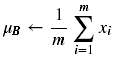
然后来求方差:
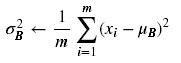
有了均值和方差,我们就可以对输入值进行归一化了:
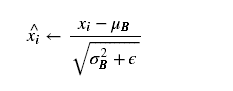 分母中我们添加了一项
 ,是为了防止分母为0,我们时实际取的值是0.001。
最后,我们还需要对归一化的值进行线性变换,使用 和
和 (它们在学习过程中会被训练)进行缩放和平移:
 这样我们就得到了最终的批量归一化的值,然后再把值传送到激活函数,比如sigmoid, tanh, ReLU, Leaky ReLU等等。
在用代码实现时,我们只需一行即可:
这样我们就得到了最终的批量归一化的值,然后再把值传送到激活函数,比如sigmoid, tanh, ReLU, Leaky ReLU等等。
在用代码实现时,我们只需一行即可:
batch_normalized_output = tf.layers.batch_normalization(linear_output, training=self.is_training)
不使用 tf.layers 包实现批量归一化
在NeuralNet 类中,我们使用的是高级封装的函数tf.layers.batch_normalization, 接下来,我使用封装的没有那么好的函数tf.nn.batch_normalization来实现批量归一化。
1)你可以使用接下来的 fully_connected 函数代替之前的函数。
def fully_connected(self, layer_in, initial_weights, activation_fn=None):
    """
    Creates a standard, fully connected layer. Its number of inputs and outputs will be
    defined by the shape of `initial_weights`, and its starting weight values will be
    taken directly from that same parameter. If `self.use_batch_norm` is True, this
    layer will include batch normalization, otherwise it will not.

    :param layer_in: Tensor
        The Tensor that feeds into this layer. It's either the input to the network or the output
        of a previous layer.
    :param initial_weights: NumPy array or Tensor
        Initial values for this layer's weights. The shape defines the number of nodes in the layer.
        e.g. Passing in 3 matrix of shape (784, 256) would create a layer with 784 inputs and 256
        outputs.
    :param activation_fn: Callable or None (default None)
        The non-linearity used for the output of the layer. If None, this layer will not include
        batch normalization, regardless of the value of `self.use_batch_norm`.
        e.g. Pass tf.nn.relu to use ReLU activations on your hidden layers.
    """
    if self.use_batch_norm and activation_fn:
        # Batch normalization uses weights as usual, but does NOT add a bias term. This is because
        # its calculations include gamma and beta variables that make the bias term unnecessary.
        weights = tf.Variable(initial_weights)
        linear_output = tf.matmul(layer_in, weights)

        num_out_nodes = initial_weights.shape[-1]

        # Batch normalization adds additional trainable variables:
        # gamma (for scaling) and beta (for shifting).
        gamma = tf.Variable(tf.ones([num_out_nodes]))
        beta = tf.Variable(tf.zeros([num_out_nodes]))

        # These variables will store the mean and variance for this layer over the entire training set,
        # which we assume represents the general population distribution.
        # By setting `trainable=False`, we tell TensorFlow not to modify these variables during
        # back propagation. Instead, we will assign values to these variables ourselves.
        pop_mean = tf.Variable(tf.zeros([num_out_nodes]), trainable=False)
        pop_variance = tf.Variable(tf.ones([num_out_nodes]), trainable=False)

        # Batch normalization requires a small constant epsilon, used to ensure we don't divide by zero.
        # This is the default value TensorFlow uses.
        epsilon = 1e-3

        def batch_norm_training():
            # Calculate the mean and variance for the data coming out of this layer's linear-combination step.
            # The [0] defines an array of axes to calculate over.
            batch_mean, batch_variance = tf.nn.moments(linear_output, [0])

            # Calculate a moving average of the training data's mean and variance while training.
            # These will be used during inference.
            # Decay should be some number less than 1. tf.layers.batch_normalization uses the parameter
            # "momentum" to accomplish this and defaults it to 0.99
            decay = 0.99
            train_mean = tf.assign(pop_mean, pop_mean * decay + batch_mean * (1 - decay))
            train_variance = tf.assign(pop_variance, pop_variance * decay + batch_variance * (1 - decay))

            # The 'tf.control_dependencies' context tells TensorFlow it must calculate 'train_mean'
            # and 'train_variance' before it calculates the 'tf.nn.batch_normalization' layer.
            # This is necessary because the those two operations are not actually in the graph
            # connecting the linear_output and batch_normalization layers,
            # so TensorFlow would otherwise just skip them.
            with tf.control_dependencies([train_mean, train_variance]):
                return tf.nn.batch_normalization(linear_output, batch_mean, batch_variance, beta, gamma, epsilon)

        def batch_norm_inference():
            # During inference, use the our estimated population mean and variance to normalize the layer
            return tf.nn.batch_normalization(linear_output, pop_mean, pop_variance, beta, gamma, epsilon)

        # Use `tf.cond` as a sort of if-check. When self.is_training is True, TensorFlow will execute
        # the operation returned from `batch_norm_training`; otherwise it will execute the graph
        # operation returned from `batch_norm_inference`.
        batch_normalized_output = tf.cond(self.is_training, batch_norm_training, batch_norm_inference)

        # Pass the batch-normalized layer output through the activation function.
        # The literature states there may be cases where you want to perform the batch normalization *after*
        # the activation function, but it is difficult to find any uses of that in practice.
        return activation_fn(batch_normalized_output)
    else:
        # When not using batch normalization, create a standard layer that multiplies
        # the inputs and weights, adds a bias, and optionally passes the result
        # through an activation function.
        weights = tf.Variable(initial_weights)
        biases = tf.Variable(tf.zeros([initial_weights.shape[-1]]))
        linear_output = tf.add(tf.matmul(layer_in, weights), biases)
        return linear_output if not activation_fn else activation_fn(linear_output)
现在的 fully_connected 函数比之前的要多许多代码,有一些重要的地方需要提醒一下:
- 展示出来我们创建各个参数的过程: gamma, beta, mean and variance。
- gamma, beta在开始时分别设置的是1和0,所以并没有进行线性变换,但是在训练过程中,使用反向传播会慢慢训练这些值,找到最合适的值。
- population mean and variance 并不会被训练,而是通过
tf.assign直接更新值。 - TensorFlow在训练期间不会自动更新
tf.assign指定的值,因为它仅基于在图中找到的连接来评估所需的操作。为了得到tf.assign指定的值,在批量归一化之前,我们需要通过with tf.control_dependencies([train_mean, train_variance]):操作。 这告诉TensorFlow,在运行with块中(with这一行以下的代码,或者说:之后的代码)的任何内容之前,它需要运行这些操作(with同一行的代码,或者说with与:之间的代码)。 - 批量归一化的计算操作是通过
tf.nn.batch_normalization来完成的. - 我们使用函数
tf.cond来判断是训练还是推断,如果第一个是True,则执行第二个函数,否则执行第三个函数。 - 我们使用函数
tf.nn.moments来计算batch的均值与偏差。
2) 如果你想实现更多细节,你可以替换 batch_norm_training:
return tf.nn.batch_normalization(linear_output, batch_mean, batch_variance, beta, gamma, epsilon)
使用这个代码:
normalized_linear_output = (linear_output - batch_mean) / tf.sqrt(batch_variance + epsilon)
return gamma * normalized_linear_output + beta
同时你也可以替换 batch_norm_inference:
return tf.nn.batch_normalization(linear_output, pop_mean, pop_variance, beta, gamma, epsilon)
使用这个代码:
normalized_linear_output = (linear_output - pop_mean) / tf.sqrt(pop_variance + epsilon)
return gamma * normalized_linear_output + beta
为什么会使用训练和推断?
在之前的函数中我们使用的是:tf.layers.batch_normalization,通过传入参数training来判断当前是否处于训练阶段:
batch_normalized_output = tf.layers.batch_normalization(linear_output, training=self.is_training)
在低版本的函数中,你或许也注意到,我们需要手动实现当前是训练还是推断阶段,但是为什么我们需要这样做呢?
假如我们不这样做,会发生什么呢?
def batch_norm_test(test_training_accuracy):
    """
    :param test_training_accuracy: bool
        If True, perform inference with batch normalization using batch mean and variance;
        if False, perform inference with batch normalization using estimated population mean and variance.
    """

    weights = [np.random.normal(size=(784,100), scale=0.05).astype(np.float32),
               np.random.normal(size=(100,100), scale=0.05).astype(np.float32),
               np.random.normal(size=(100,100), scale=0.05).astype(np.float32),
               np.random.normal(size=(100,10), scale=0.05).astype(np.float32)
              ]

    tf.reset_default_graph()

    # Train the model
    bn = NeuralNet(weights, tf.nn.relu, True)

    # First train the network
    with tf.Session() as sess:
        tf.global_variables_initializer().run()

        bn.train(sess, 0.01, 2000, 2000)

        bn.test(sess, test_training_accuracy=test_training_accuracy, include_individual_predictions=True)
batch_norm_test(True)
100%|██████████| 2000/2000 [00:03<00:00, 514.57it/s]


With Batch Norm: After training, final accuracy on validation set = 0.9527996778488159
---------------------------------------------------------------------------
With Batch Norm: Accuracy on full test set = 0.9503000974655151
200 Predictions: [8, 8, 8, 8, 8, 8, 8, 8, 8, 8, 8, 8, 8, 8, 8, 8, 8, 8, 8, 8, 8, 8, 8, 8, 8, 8, 8, 8, 8, 8, 8, 8, 8, 8, 8, 8, 8, 8, 8, 8, 8, 8, 8, 8, 8, 8, 8, 8, 8, 8, 8, 8, 8, 8, 8, 8, 8, 8, 8, 8, 8, 8, 8, 8, 8, 8, 8, 8, 8, 8, 8, 8, 8, 8, 8, 8, 8, 8, 8, 8, 8, 8, 8, 8, 8, 8, 8, 8, 8, 8, 8, 8, 8, 8, 8, 8, 8, 8, 8, 8, 8, 8, 8, 8, 8, 8, 8, 8, 8, 8, 8, 8, 8, 8, 8, 8, 8, 8, 8, 8, 8, 8, 8, 8, 8, 8, 8, 8, 8, 8, 8, 8, 8, 8, 8, 8, 8, 8, 8, 8, 8, 8, 8, 8, 8, 8, 8, 8, 8, 8, 8, 8, 8, 8, 8, 8, 8, 8, 8, 8, 8, 8, 8, 8, 8, 8, 8, 8, 8, 8, 8, 8, 8, 8, 8, 8, 8, 8, 8, 8, 8, 8, 8, 8, 8, 8, 8, 8, 8, 8, 8, 8, 8, 8, 8, 8, 8, 8, 8, 8]
Accuracy on 200 samples: 0.05
如您所见,网络每次都猜到了相同的值!但是为什么?因为在训练期间,每次传入一个样本(比如一张图片),那么得到的均值就是当前样本的值,方差为0,所以进过归一化操作后,值都会变为0(你可以查看之前的等式,归一化的具体实现),那么无论传入什么值,在网络中的输入值都是0,所以得到的结果都是一样的。
为了克服这个问题,当我们执行推理时,不是让它使用它们自己的均值和方差来“归一化”所有值,而是使用它在训练时计算的总体均值和方差的估计。
batch_norm_test(False)
100%|██████████| 2000/2000 [00:03<00:00, 511.58it/s]


With Batch Norm: After training, final accuracy on validation set = 0.9577997326850891
---------------------------------------------------------------------------
With Batch Norm: Accuracy on full test set = 0.953700065612793
200 Predictions: [7, 2, 1, 0, 4, 1, 4, 9, 6, 9, 0, 8, 9, 0, 1, 5, 9, 7, 3, 4, 9, 6, 6, 5, 4, 0, 7, 4, 0, 1, 3, 1, 3, 6, 7, 2, 7, 1, 2, 1, 1, 7, 4, 2, 3, 5, 1, 2, 4, 4, 6, 3, 5, 5, 6, 0, 4, 1, 9, 5, 7, 8, 9, 3, 7, 4, 6, 4, 3, 0, 7, 0, 2, 9, 1, 7, 3, 2, 9, 7, 7, 6, 2, 7, 8, 4, 7, 3, 6, 1, 3, 6, 4, 3, 1, 4, 1, 7, 6, 9, 6, 0, 5, 4, 9, 9, 2, 1, 9, 4, 8, 7, 3, 9, 7, 4, 4, 4, 9, 2, 5, 4, 7, 6, 7, 9, 0, 5, 8, 5, 6, 6, 5, 7, 8, 1, 0, 1, 6, 4, 6, 7, 3, 1, 7, 1, 8, 2, 0, 4, 9, 8, 5, 5, 1, 5, 6, 0, 3, 4, 4, 6, 5, 4, 6, 5, 4, 5, 1, 4, 4, 7, 2, 3, 2, 7, 1, 8, 1, 8, 1, 8, 5, 0, 8, 9, 2, 5, 0, 1, 1, 1, 0, 9, 0, 3, 1, 6, 4, 2]
Accuracy on 200 samples: 0.97
如你所见,现在我们使用估计的总体均值和方差,我们得到97%的精度。
其他网络类型的注意事项
本例子演示了具有完全连接层的标准神经网络中的批量归一化。您也可以在其他类型的网络中使用批量归一化,但有一些特殊的注意事项。
ConvNets
卷积层是由多个feature maps构成,每个feature map共享权重,由于这些差异,批量归一化卷积层需要每个特征映射而不是层中的每个节点的批量/总体均值和方差。
通常,我们可以通过下面的代码来计算batch mean and variance:
batch_mean, batch_variance = tf.nn.moments(linear_output, [0])
但是在卷积层中,我们需要注意:
batch_mean, batch_variance = tf.nn.moments(conv_layer, [0,1,2], keep_dims=False)
第二个参数, [0,1,2], 告诉 TensorFlow在一个batch上面 计算每个feature map的均值与偏差。(三个轴分别是: batch, height, and width.) 设置keep_dims 为 False 是为了让tf.nn.moments 不要返回与输入相同的维度,确保我们得到的是每个feature map的均值与偏差。
RNNs
批量归一化也可以用作循环神经网络中,你可以参考这篇论文Recurrent Batch Normalization. 它是在每个时间步长计算均值与偏差,而不是每一层。你也可以在这上面找到例子this GitHub repo.